Mathematics
Right triangle
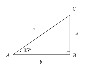
A right triangle with an angle marker and attached vertex and side labels.
Download SVGStart with a ready-made scientific figure, then adjust its geometry and labels in Mathcha. Browse the library below, search by name or description, or filter by field. Open any preview for a full-size vector image, or download its SVG.
Labels use the document’s text and math fonts. Resizing changes the drawing while keeping label sizes fixed. Expand Label settings to change text/math sizes, hide labels, or choose Rotate with figure; labels stay upright by default.
The gallery shows each family’s default construction with its default labels. The editor contains the editable figure and its other presets. These are schematic starting points; plotted curves and diagrams are not substitutes for measured data or a scientific simulation.
210 of 210 figure families
Mathematics
A right triangle with an angle marker and attached vertex and side labels.
Download SVG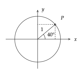
Mathematics
A circle with a radius, angle, and horizontal and vertical projections.
Download SVG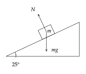
Physics
A frictionless block with weight and normal-force directions. Arrow lengths are schematic.
Download SVG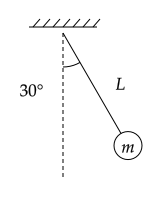
Physics
A pendulum with an equilibrium guide, attached length label, and angle marker.
Download SVG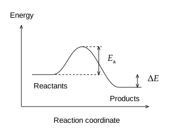
Chemistry
A schematic single-step energy profile. Negative energy change places products below reactants.
Download SVG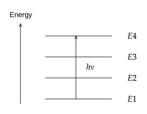
Chemistry
Equally spaced schematic levels with a transition from the lowest to highest level.
Download SVG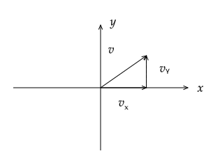
Mathematics
A vector and its signed Cartesian components. The angle is measured counterclockwise from the positive x-axis.
Download SVG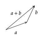
Mathematics
Two vectors and their resultant, with triangle or parallelogram construction. Arrow lengths share one relative scale.
Download SVG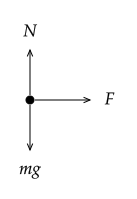
Physics
External forces on a particle or block. Directions and arrow lengths are user specified; equilibrium is not assumed.
Download SVG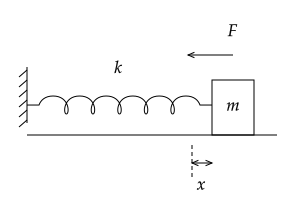
Physics
A spring attached to a sliding mass. Displacement changes the spring length; force arrow indicates the restoring direction.
Download SVG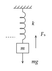
Physics
A hanging spring and mass. Extension is measured from the indicated reference level; arrows show weight and spring force schematically.
Download SVG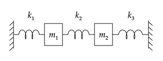
Physics
Two masses between fixed supports, connected by three springs. Mass offsets change the individual spring lengths.
Download SVG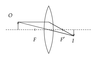
Physics
Principal rays for converging or diverging thin lenses. Image position follows the thin-lens equation; dashed extensions locate virtual images.
Download SVG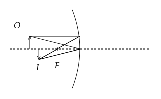
Physics
Paraxial rays for concave or convex mirrors. Solid rays show real paths; dashed extensions locate virtual images. Distances use one scale.
Download SVG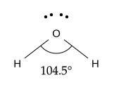
Chemistry
H₂O: two single bonds and two lone pairs on oxygen. The adjustable H–O–H angle defaults to 104.5°.
Download SVG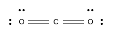
Chemistry
CO₂: linear O=C=O with two lone pairs on each oxygen. Bond/electron controls also support user-authored schematics.
Download SVG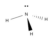
Chemistry
NH₃: three single bonds and one nitrogen lone pair. Solid and hashed wedges indicate a schematic pyramidal arrangement.
Download SVG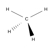
Chemistry
CH₄: four single bonds and no carbon lone pairs. Wedges indicate a schematic tetrahedral arrangement, not a measured projection.
Download SVG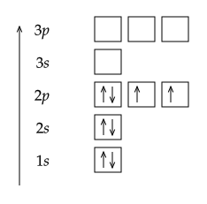
Chemistry
Ground-state filling of 1s–3p for one to eighteen electrons. Degenerate p orbitals fill singly before pairing, following Hund’s rule.
Download SVG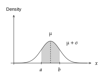
Statistics
A sampled normal probability density with an interval or tail shaded. The mean and standard deviation change the curve; shaded bounds are x-values, not probabilities.
Download SVG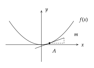
Mathematics
A function with its analytic tangent or a secant through two points. The dashed slope triangle follows the selected line.
Download SVG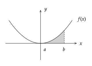
Mathematics
The shaded signed region between a selected function and the x-axis. Endpoints are ordered automatically; the figure does not report a numerical integral.
Download SVG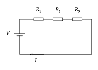
Engineering
A complete source-and-resistor loop using Mathcha’s circuit symbols. Labels and current direction are schematic; this is not a circuit solver.
Download SVG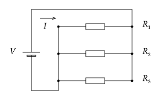
Engineering
A source feeding two to four parallel branches. Junction dots and connected terminals follow the selected branch count.
Download SVG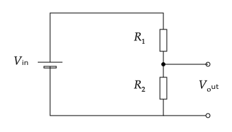
Engineering
Two series resistors with an output tap referenced to the lower rail. Component values are editable labels; no output voltage is calculated.
Download SVG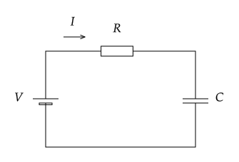
Engineering
A source, resistor and capacitor in series. The capacitor voltage and current labels can be edited for charging or discharging discussions.
Download SVG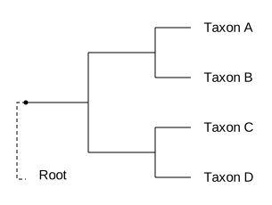
Biology
A rooted tree with four or eight editable taxa and balanced or ladder branching. Branch lengths are schematic and do not imply elapsed time.
Download SVG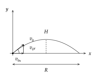
Physics
An ideal ballistic trajectory without air resistance. Angle, speed, launch height and gravity determine the path, apex and landing point; one common spatial scale is used.
Download SVG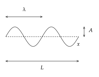
Physics
A traveling-wave snapshot or standing-mode envelope. Pipe curves show displacement, not pressure. Open ends are displacement antinodes; closed ends are nodes. Dashed curves show the opposite extreme.
Download SVG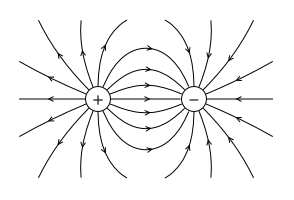
Physics
Point charge, equal-and-opposite dipole, or ideal parallel-plate field. Arrows follow the force on a positive test charge. Dipole paths are integrated from Coulomb's field; plates omit fringing.
Download SVG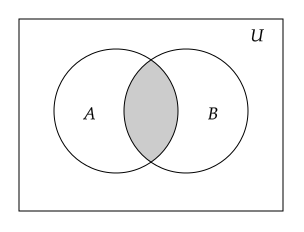
Mathematics
Two or three sets inside a universal set. Shading is built from disjoint circular regions, so intersections and complements export consistently. A and B operations include their portions inside C.
Download SVG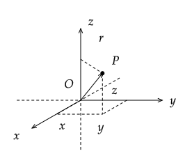
Mathematics
A two-dimensional projection of three-dimensional axes and a signed point/vector. Dashed component guides follow the coordinates. Projection changes the view, not the coordinate values.
Download SVG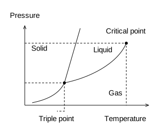
Chemistry
A schematic pressure–temperature phase diagram for a pure substance. Typical and water-like presets change the melting-line slope. Positions are relative, not experimental data or a calibrated equation of state.
Download SVG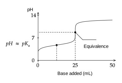
Chemistry
Strong or weak monoprotic acid titrated with a strong base at 25 °C. Curves solve mass and charge balance including water ionization, using ideal concentrations. The view spans zero to twice the equivalence volume.
Download SVG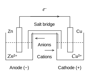
Chemistry
A schematic galvanic cell with oxidation at the anode and reduction at the cathode. Electron arrows run through the external circuit from anode to cathode; ions carry charge through the salt bridge. Labels do not calculate electrode potentials.
Download SVG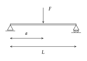
Engineering
A schematic simply supported, cantilever or overhanging beam. Place point loads, uniform distributed loads and applied moments. Load arrows and reaction arrows are annotations; reactions, stress and deflection are not solved.
Download SVG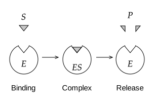
Biology
A schematic enzyme–substrate sequence, with competitive and noncompetitive inhibition presets. Shapes illustrate binding roles, not molecular structures; noncompetitive inhibition is simplified to an inactive bound complex.
Download SVG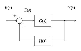
Engineering
Editable signal-flow presets: negative/positive feedback, a cascade, and feedback with an output disturbance. Blocks and transfer functions are annotations, not an automatic algebra or stability solver.
Download SVG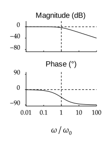
Engineering
Exact normalized first/second-order low-pass and high-pass responses. Frequency is ω/ω₀ on a logarithmic axis; gain is dB. Positive damping excludes singular undamped resonance. No arbitrary transfer-function solver or stability margins.
Download SVG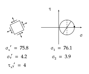
Engineering
Tension-positive plane stress with positive τxy acting upward on the +x face. A counterclockwise element rotation θ maps to −2θ on the circle with shear positive upward. All stresses share the same user-chosen unit; deformation and strain are not calculated.
Download SVG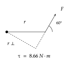
Physics
A force at an angle to a lever, a fixed ideal pulley, or a wheel rolling without slipping. Torque is rF sinθ; rolling uses v=ωR. Pulley masses and tensions are editable annotations; no pulley acceleration or friction is inferred.
Download SVG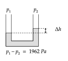
Physics
U-tube pressure difference, ideal equal-height hydraulic pistons, and a horizontal ideal Bernoulli/continuity pipe. Area ratio drives piston/pipe diameters by its square root and flow speed by continuity. Steady incompressible flow, negligible losses; schematic lengths are not a pressure or velocity scale.
Download SVG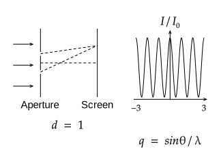
Physics
Ideal double-slit interference, single-slit diffraction, and an N-slit grating. Plot uses q=sinθ/λ with distances in common relative units. Slit/grating interference assumes point-like slits; only the single-slit mode includes the finite-width envelope. Far field, monochromatic coherent illumination.
Download SVG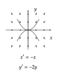
Mathematics
Quick Cartesian illustrations of six fixed linear systems: stable/unstable node, saddle, center, stable/unstable spiral. Curves are analytic solutions and arrows show increasing time. Use the existing Poincaré-disc plot tool for user-defined polynomial systems and numerical trajectories.
Download SVG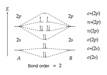
Chemistry
Homonuclear diatomic valence MO diagrams: a 1s pair, or 2s/2p levels with B₂–N₂ or O₂–Ne₂ ordering. Electrons fill degenerate π orbitals singly before pairing. Atomic side levels are unoccupied references. Relative energies are schematic; labels/occupancy do not infer atom identity, charge, or a general molecular wavefunction.
Download SVG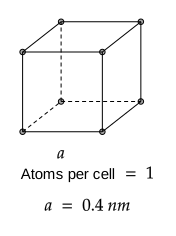
Chemistry
Simple, body-centered and face-centered cubic lattice-point diagrams in oblique projection. Optional (100), (110), (111) planes show geometric intercepts. Dots mark atom centers, not space-filling radii. Atom count includes boundary sharing; no arbitrary crystal basis, diffraction simulation or surface chemistry.
Download SVG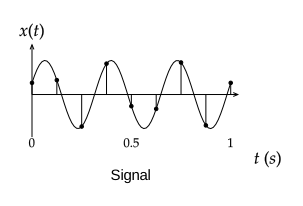
Signal processing
A sinusoid sampled uniformly over one second; dashed alias uses f − fs·round(f/fs), so it agrees at every sample including phase. Spectrum mode shows triangular bandlimited replicas at integer multiples of fs, not a computed Fourier transform. Frequencies are Hz; exact Nyquist sampling can lose phase information.
Download SVG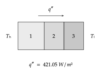
Engineering
Steady one-dimensional conduction through two or three perfect-contact planar layers of unit area. R″ = L/k (m²·K/W); q″ = (Th−Tc)/ΣR″. Profiles use continuous interface temperatures; the network uses area-specific resistances. No convection, contact resistance or internal generation.
Download SVG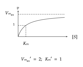
Biochemistry
Steady-state Michaelis–Menten initial rates with v = Vmax[S]/(Km+[S]). Competitive inhibition increases apparent Km by α=1+[I]/Ki; pure noncompetitive inhibition divides Vmax by α with unchanged Km. Solid is uninhibited, dashed inhibited. Concentration/rate units are arbitrary but consistent; no data fitting or mixed inhibition.
Download SVG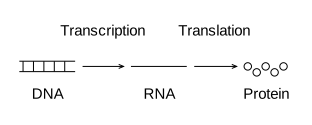
Molecular biology
Editable central-dogma, three-exon splicing and simple transcriptional-regulation schematics. Splicing retains all three exons and removes both introns. Regulation uses an arrow for activation and a blunt end for repression. Sequence lengths and molecular sizes are schematic; no sequence translation or gene-network simulation.
Download SVG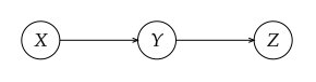
Statistics
Directed chain, common-cause fork, collider, three-step hidden Markov model and iid plate notation. Shaded nodes are observed; unshaded nodes are latent/unobserved. HMM observations are shaded and the plate has a shared unobserved parameter. These are editable graph schematics, not probability inference or causal-identification results.
Download SVG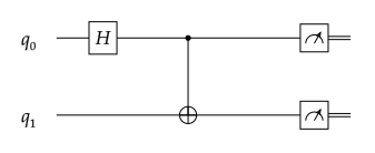
Quantum information
Left-to-right gate schematics: a single-qubit gate sequence, Bell preparation (H then CNOT) and GHZ preparation (H then chained CNOTs). Filled control dots and ⊕ targets use standard controlled-X notation. Optional meters terminate quantum wires in double classical wires. Labels are editable; no state-vector simulation or hardware mapping.
Download SVG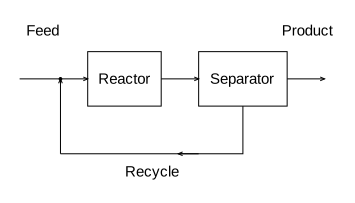
Chemical engineering
Reactor–separator flow with optional recycle/purge, or a two-stream parallel/counterflow heat-exchanger schematic. Arrowheads specify stream directions; a recycle mixer joins fresh feed upstream of the reactor. Equipment and stream labels are editable. No mass/energy balance, process simulation or detailed P&ID symbols.
Download SVG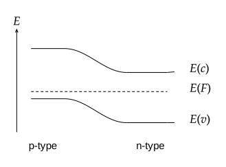
Semiconductor physics
Schematic conductor/semiconductor/insulator bands, an equilibrium p–n band diagram, and abrupt-junction depletion charge/field profiles. At equilibrium EF is flat; Ec and Ev bend together. Wp/Wn=ND/NA and charge-density heights balance integrated charge. Axes are normalized; no material-specific Poisson solution, applied bias or carrier statistics.
Download SVG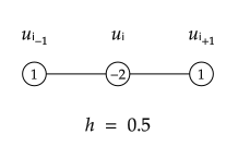
Applied mathematics
Uniform-grid centered second-derivative stencils (three-point 1D or five-point 2D), a finite-volume cell with outward face fluxes, and a small structured mesh with left/right Dirichlet and top/bottom zero-normal-gradient boundaries. Stencil weights must be divided by h². These are annotations, not a PDE solver or arbitrary mesh generator.
Download SVG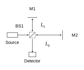
Optics
Top-view Michelson and Mach–Zehnder layouts with beam splitters, mirrors, source and detector. Michelson outgoing/return arms share paths; a two-headed arrow denotes the round trip. Mach–Zehnder paths run through two splitters and two turning mirrors. Geometry is schematic; no interference simulation, polarization or phase calculation.
Download SVG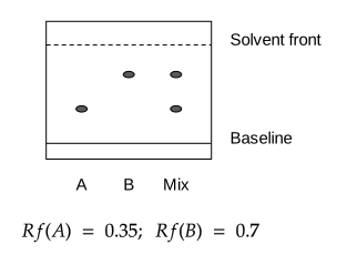
Analytical chemistry
TLC reference lanes A/B and a mixture show two user-specified Rf values, measured from the baseline to a common solvent front. Column mode is a packed-bed schematic with two separated bands and a collection vessel; it does not predict elution from TLC Rf, solvent chemistry or experimental data.
Download SVG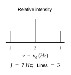
Spectroscopy
Ideal first-order coupling to n equivalent spin-½ neighbors: n+1 equally spaced lines with binomial intensities. Frequency decreases to the right; J is in Hz. Lorentzian broadening sums the lines, normalized to the tallest isolated component, not the total peak height. No molecular assignment, strong coupling, experimental data or quantitative integration.
Download SVG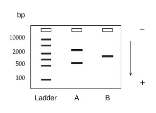
Laboratory biology
Schematic DNA agarose or denaturing-protein SDS-PAGE lanes, with an illustrative ladder and user-specified sizes. Smaller fragments/proteins migrate farther, using a logarithmic size-to-position mapping. Lane A has one/two bands; lane B has one. Ladder positions/intensities are illustrative, not a commercial marker, measured gel, identification or quantification.
Download SVG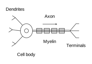
Neuroscience
Schematic neuron, chemical synapse and illustrative action-potential waveform. Presynaptic vesicles release transmitter across a cleft toward postsynaptic receptors. Waveform controls set rest/peak voltage; threshold is −55 mV and the undershoot is below rest. Time/shape are illustrative, not a Hodgkin–Huxley model, recording or anatomical reconstruction.
Download SVG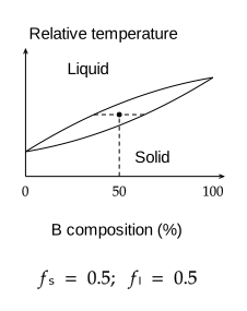
Materials science
Illustrative temperature–composition diagrams, not real-alloy data. Isomorphous boundaries are monotone quadratics with analytic tie-line intersections. The eutectic model has pure A/B solids and no solid solubility. Fractions conserve composition; at the three-phase eutectic temperature they are not uniquely determined and no fractions are reported.
Download SVG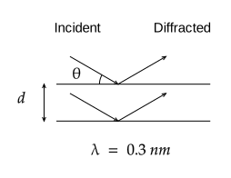
Crystallography
Bragg reflection uses nλ=2d sinθ. Reciprocal-space modes use the crystallographic convention a*=1/a (no 2π), with b*/a* set by the aspect ratio. The 2D Ewald construction selects G=(−a*,b*) and calculates its elastic wavelength; the circle passes exactly through O and G. Plane lengths and lattice drawings are schematic; no structure factors or full diffraction pattern.
Download SVG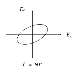
Optics
Transverse Ex=cos(t), Ey=A cos(t+δ) at one fixed point: linear, circular and elliptical presets, with an arrow for increasing time. Filter mode uses ideal polarizer/analyzer symbols and Malus's law: cos²θ for input aligned to the first polarizer, or ½cos²θ for unpolarized input. The drawing is schematic and does not simulate wave plates or scattering.
Download SVG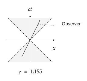
Relativity
One spatial dimension, with equal x and ct scales. Light rays have slopes ±1. Primed axes satisfy ct=βx and x=βct; γ=1/√(1−β²). Simultaneity mode places A/B at ct′=0.8, so ct=0.8/γ+βx. Light-cone shading and observer worldlines are schematic, with subluminal speeds; no gravity or curved spacetime.
Download SVG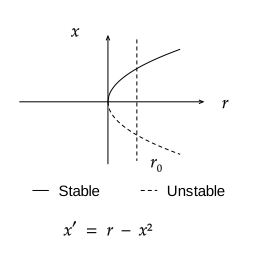
Applied mathematics
Equilibria versus parameter r for x′=r−x², x′=rx−x², x′=rx−x³ and x′=rx+x³. Solid branches are stable and dashed branches unstable, from the sign of ∂x′/∂x. The guide marks a selected parameter, not a trajectory. These are canonical analytic diagrams, not numerical continuation or an arbitrary nonlinear-system solver.
Download SVG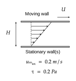
Fluid mechanics
Ideal steady, fully developed laminar Newtonian flow: plane Couette, plane Poiseuille and a pipe diametral section. Arrow lengths show u/umax. Plane gap is H; pipe diameter is 2R. Pressure drive G=−dp/dx>0. Calculated umax and wall-shear magnitude use μ in mPa·s and lengths in mm; density is not required. No turbulence, entrance effects or CFD.
Download SVG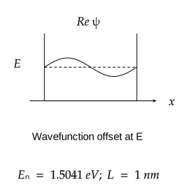
Quantum mechanics
Electron in an infinite 1D well, a semi-infinite step with E<V, or a finite square barrier with E<V. The box energy is 0.37603 n²/L² eV for L in nm. Scattering uses exact stationary matching, unit incident amplitude and the real part at a chosen phase; curves are vertically offset at E, not additional energy. The finite-barrier transmission includes interface reflections. No arbitrary-potential solver or wave-packet dynamics.
Download SVG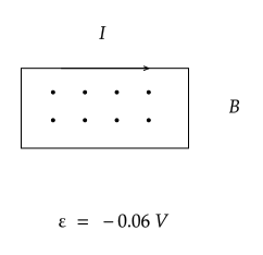
Electromagnetism
Changing uniform flux through N identical turns, a magnet approaching/receding from a side-view coil, or a rod sliding on rails. Dot/cross fields point out of/into the page. Loop arrows follow Lenz's law; magnet mode shows the induced axial field rather than an ambiguous side-view current. Flux mode uses ε=−NA dB/dt and rod mode |ε|=Bℓ|v|. Ideal circuits; no resistance/current magnitude or field solver.
Download SVG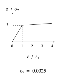
Materials mechanics
Bilinear elastic/plastic engineering stress–strain response, Maxwell creep, Kelvin–Voigt creep or Maxwell stress relaxation. The plastic tangent is a fraction of the elastic modulus. Linear-viscoelastic models use τ=η/E, MPa and MPa·s. Creep strain is normalized by σ₀/E; relaxation stress by its initial value. Axes t/τ make model comparisons explicit. Ideal constitutive models, not measured material data or failure prediction.
Download SVG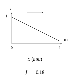
Mass transport
Steady one-dimensional diffusion through a layer, or transient spreading from an instantaneous planar sheet in an infinite medium. The sheet has amount per area Q=1 and c(x,t)=Q exp(−x²/4Dt)/√(4πDt), preserving total amount on the infinite line. Displayed profiles are at t, 2t and 4t with one common concentration scale. D is mm²/s, x is mm; plotted tails extend to ±3√(8Dt). No finite-boundary, reaction or convection solver.
Download SVG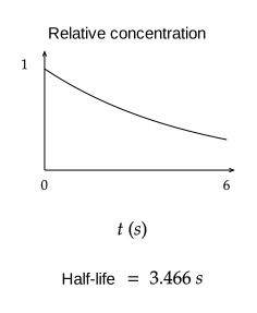
Chemical kinetics
Zero-, first- and second-order single-reactant kinetics, or irreversible first-order A→B→C. Curves use relative concentrations and seconds. k has units M/s, 1/s or 1/(M·s) for order 0, 1 or 2; chain constants use 1/s. Zero-order concentration stops at zero. The chain handles k₁=k₂ analytically and conserves A+B+C. No reversible networks or arbitrary kinetic solver.
Download SVG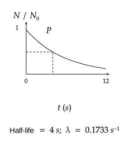
Nuclear physics
Single radioactive parent or a unit-branching parent→radioactive daughter→stable chain, initially all parent. Curves show nuclide amount relative to initial parent, or activity relative to initial parent activity. Bateman's two-member solution includes the equal-half-life limit. Half-lives and time are seconds. A marker shows the parent half-life when it lies within the view. No branching networks, dose calculation or isotope database.
Download SVG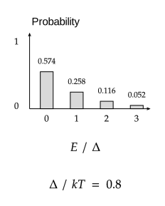
Statistical mechanics
Four nondegenerate equally spaced levels with normalized Boltzmann probabilities, or ideal Fermi–Dirac/Bose–Einstein mean occupations. Continuous modes use x=(E−μ)/(kT₀), k the Boltzmann constant, and adjustable T/T₀. Fermi mode includes the zero-temperature step. Bose mode plots x≥0.3 and rescales its vertical axis to the actual occupation there, avoiding the divergent endpoint. No density-of-states integral or condensate calculation.
Download SVG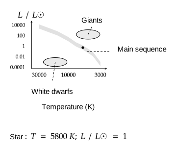
Stellar astronomy
Schematic Hertzsprung–Russell diagram: temperature decreases to the right on a logarithmic axis; luminosity is logarithmic from 10⁻⁴ to 10⁴ solar units. Main-sequence, giant and white-dwarf regions are illustrative, not fitted evolutionary tracks or classification boundaries. An independently editable star marker uses its actual temperature and luminosity coordinates. No stellar simulation, catalogue lookup or inferred age/mass.
Download SVG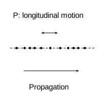
Seismology
Longitudinal P and transverse S particle-motion schematics; an illustrative seismogram with physically placed arrivals; or homogeneous-medium travel-time lines. Distances are km and velocities km/s, with vP>vS throughout the controls. Arrival times equal distance/velocity. Trace pulse shape and amplitude are illustrative, not a recorded waveform, magnitude estimate or Earth ray-tracing/inversion model.
Download SVG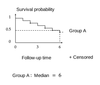
Biostatistics and reliability
Kaplan–Meier steps for one/two cohorts at six equally spaced times. Events precede censoring at ties; + marks one or more censors after the event drop. Cohorts start with 60–200 subjects and each interval allows ≤6 events/≤3 censors, ensuring positive risk sets. Remaining subjects stay at risk at the view endpoint. Median is the first time survival ≤0.5, or not reached. Grouped counts only; no confidence intervals, Cox fitting or clinical inference.
Download SVG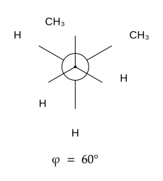
Organic chemistry
Newman projection with independent front/back substituents and a 0–180° dihedral; a single-center Fischer projection whose horizontal bonds point toward the viewer; and a perspective cyclohexane chair with one axial or equatorial substituent. Chair options designate alternative placements, not a stereochemistry-preserving ring-flip simulation. Editable chemical labels; no CIP assignment or conformational-energy calculation.
Download SVG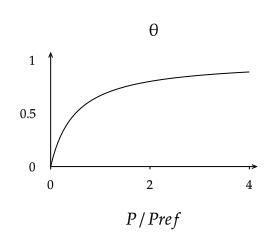
Surface science
Ideal Langmuir fractional monolayer coverage θ=KP/(1+KP), empirical Freundlich q/qref=(P/Pref)^(1/n), or BET multilayer uptake with 0≤P/P₀≤0.8. Axes show normalized pressure and coverage/uptake. BET excludes the saturation singularity and is illustrative rather than a surface-area fit; no data fitting or pore-size inference.
Download SVG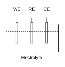
Electrochemistry
A labeled three-electrode cell, a deliberately schematic cyclic-voltammetry pair with scan directions, and the exact ideal Rₛ+(Rct∥Cdl) Nyquist semicircle. CV peak curves illustrate annotation only and are not a reversible diffusion-limited current model. Nyquist uses −Im Z on the vertical axis, with high frequency at the left intercept; no Warburg, fitting or electrochemical kinetics solver.
Download SVG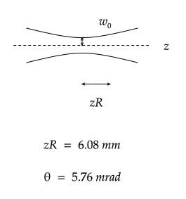
Photonics
Paraxial M²=1 Gaussian beam envelope with w₀ measured at 1/e² intensity, zR=πw₀²/λ and far-field half-angle λ/(πw₀). Focused mode applies the exact thin-lens q transform q′=q/(1−q/f); positive waist distance means downstream of the lens, negative means upstream. Coordinates use incident zR and a shared vertical drawing scale; transverse and longitudinal distances are not to scale. No aberrations or resonator stability solver.
Download SVG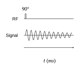
Magnetic resonance
Ideal pulse–acquire, Hahn spin echo and inversion-recovery spin echo, with RF and receiver-signal tracks on one time scale. Echo occurs TE after the 90° pulse; the refocusing 180° pulse is at TE/2. Inversion recovery places a 180° pulse TI before excitation. Signal envelopes use exp(−TE/T₂) and the signed long-TR factor 1−2exp(−TI/T₁). Carrier oscillations and echo width are illustrative; no spatial MRI gradient design or Bloch simulator.
Download SVG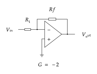
Analog electronics
Ideal negative-feedback inverting/non-inverting amplifiers, voltage follower, two-input inverting summer and inverting integrator. Gain coefficients use positive kΩ resistance values; integrator reports RC in ms for C in µF. The voltage follower has its signal on + and output feedback on −. Supply rails are omitted. These are topology/ideal-gain presets, not rail, bandwidth, stability or time-domain simulation.
Download SVG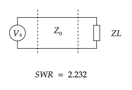
RF engineering
Lossless source–line–load schematic, voltage standing-wave magnitude versus distance from the load in wavelengths, or a reduced normalized-impedance Smith grid. Γ=(ZL−Z₀)/(ZL+Z₀), ZL=R+jX with R≥0. Smith marker uses the same exact Γ; upper half is inductive. SWR is infinite for |Γ|=1 and one for a matched load. No lossy line, matching-network synthesis or S-parameter fitting.
Download SVG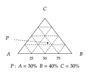
Mixtures and geochemistry
Equilateral A–B–C composition triangle with quarter-fraction guides, a composition point P, or mixing of endmembers P and Q. Nonnegative input weights are normalized to sum to one; three zero weights mean equal thirds. Mix parameter is the mass/mole fraction of Q on the chosen consistent composition basis. Markers and displayed fractions use the same barycentric construction. No phase boundaries, phase-equilibrium solver or inferred tie lines.
Download SVG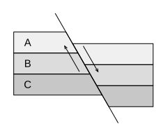
Structural geology
Three labeled stratigraphic units offset by a right-dipping normal/reverse fault, or smoothly layered anticline/syncline sections. Normal-fault hanging wall (right block) moves down; reverse-fault hanging wall moves up. Dip is a geometric section angle and throw is a drawing-coordinate displacement, not a measured length. Fold curves are controlled schematic layers; no balanced-section reconstruction, tectonic stress inversion or stereonet solver.
Download SVG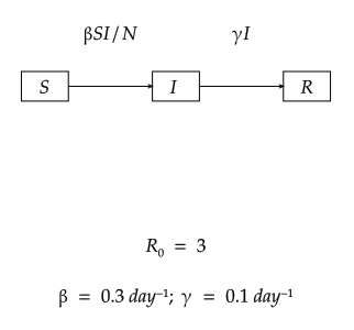
Epidemiology
Closed-population SIR, SEIR, SIR with S→R vaccination, and SIRS with R→S waning immunity. Flow labels use incidence βSI/N, exposed progression σE and recovery γI. Optional basic R₀=β/γ assumes homogeneous mixing, a fully susceptible population, no vital dynamics and eventual progression of exposed individuals. Basic R₀ is not a vaccination-adjusted effective reproduction number. These are editable model schematics, not outbreak forecasts or fitted trajectories.
Download SVG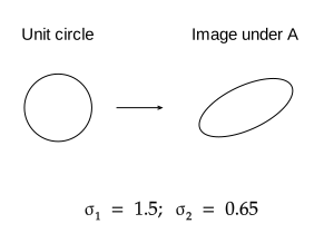
Linear algebra
Exact two-dimensional rotation/stretch constructions: A=R(α)diag(σ₁,σ₂)R(β), its three stages, a symmetric eigensystem R(α)diag(σ₁,σ₂)R(α)ᵀ, or orthogonal projection of v=(1.5,1) onto a line. Singular values are nonnegative and may be zero; their order is user-controlled. This constructs matrices from factors, rather than decomposing arbitrary matrix input. No PCA inference or numerical eigensolver.
Download SVG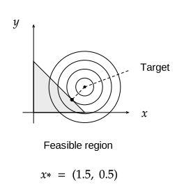
Optimization
A quadratic objective projected onto the nonnegative triangle x+y≤b, a linear objective maximized on a unit circle, or five exact gradient-descent steps for f=½[(x−1.5)²+4(y−1.5)²]. The triangle optimum is the exact Euclidean projection, including vertex and feasible-target cases. Circle arrows show its outward normal; descent uses a bounded stable step. These are fixed analytic examples, not an arbitrary optimization solver.
Download SVG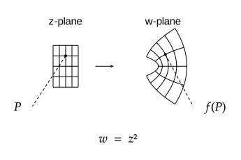
Complex analysis
Paired z and w planes map the same right-half-plane grid under w=z², w=1/z or w=exp(z). Domain 0.4≤Re z≤1.6 and −1≤Im z≤1 avoids the reciprocal pole and the critical point of z²; exp is injective on this strip. Output panels have map-specific display scales. Grid images are sampled curves, not a general conformal-domain solver or a Riemann-surface renderer.
Download SVG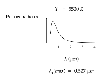
Thermal radiation
Planck spectral radiance per wavelength from 0.3 to 4 µm at 2500–9000 K. Radiance is normalized to the hottest displayed curve's peak, with one shared vertical scale. Dashed/solid curves compare temperatures. Wien peaks use λmax T=2897.771955 µm K; total emitted-power ratio is (T₁/T₂)⁴. Ideal blackbody only; no emissivity fit, frequency-axis conversion or material spectrum.
Download SVG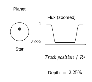
Observational astronomy
Uniform-brightness stellar disk and exact circle-overlap transit flux, paired with a zoomed light curve along a straight projected track. Radius ratio and impact parameter determine depth, grazing and no-transit cases. Wobble mode pairs schematic circular barycentric orbits with v=K sin(2πphase), positive receding. Orbital drawing sizes are illustrative; no limb darkening, eccentric fitting, transit-duration/orbit inference or planet-mass estimation.
Download SVG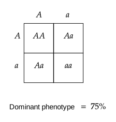
Genetics
Monohybrid crosses with selectable AA/Aa/aa parents; independent-locus AaBb×AaBb dihybrid grid; and fixed two-generation autosomal recessive/dominant pedigrees. Punnett cells keep dominant alleles first and calculate Mendelian genotype/phenotype probabilities under complete dominance. Pedigree dark symbols mean affected and half shading denotes known recessive carriers. Trait symbols are editable, but no arbitrary pedigree inference, linked-gene recombination or clinical risk prediction is performed.
Download SVG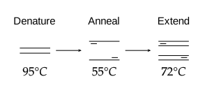
Molecular laboratory
PCR denaturation/primer-annealing/extension schematic, repeated temperature program, or illustrative qPCR fluorescence curves. qPCR uses a sigmoid calibrated so the chosen Cq is exactly at the selected threshold; a second trace has an explicit cycle shift. Fluorescence is normalized, not inferred from a sample. No sequence design, experimental curve fitting, assay validation or clinical interpretation.
Download SVG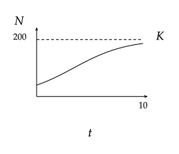
Population ecology
Exact logistic N(t)=K/[1+(K/N₀−1)e^(−rt)] for 0<N₀<K, the corresponding density-dependent growth parabola, or Lotka–Volterra positive-population nullclines. Predator–prey axes are normalized by x*=c/d and y*=a/b; arrows show quadrant signs with standardized lengths, not speeds or numerically integrated trajectories. No stochastic ecology, empirical fitting or general nonlinear ODE simulation.
Download SVG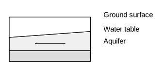
Hydrogeology
Unconfined/confined aquifer cross-sections, a saturated Darcy column Q=KA(h₁−h₂)/L, or an ideal confined steady pumping-well drawdown s(r)=Q ln(R/r)/(2πKb). Well curves are normalized vertically to display the cone; the reported well drawdown is in metres. Sections and piezometer heights are schematic. Homogeneous horizontal flow and a specified outer radius; no transient Theis solution, multiple-well superposition or groundwater simulation.
Download SVG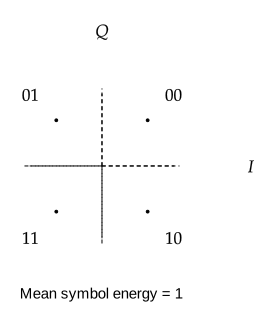
Digital communications
BPSK, QPSK, 8-PSK and square 16-QAM symbol sets with unit mean symbol energy, editable cyclic/axis Gray bit labels, optional nearest-neighbor decision boundaries and a received-point marker. PSK rotation is applied to both symbols and decision sectors; 16-QAM uses levels ±1,±3 divided by √10. Spacing expands to preserve fixed-size native bit labels. Decision lines are ideal equal-prior AWGN boundaries; no channel, bit-error estimator or waveform/eye-diagram simulation.
Download SVG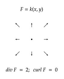
Vector calculus
Planar fields F=k(x,y), F=-k(x,y), and F=k(-y,x) show source, sink and circulation with their exact divergence and out-of-plane curl. Arrows share one relative scale. Surface mode is an oriented sheet of area A in a uniform field of magnitude k, with flux k A cos(theta). These are analytic constructions, not an arbitrary field/surface-integral solver.
Download SVG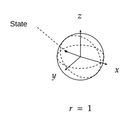
Quantum-state geometry
Orthographic Bloch-sphere projection with unit axes, equator, a meridian and a state vector. Pure-state length is one; mixed-state length is r in [0,1]. Z-measurement probabilities are p(0)=(1+r cos(theta))/2 and p(1)=1-p(0). Angles are spherical coordinates; the projected sphere is not a multiqubit state or a general dynamics/tomography simulation.
Download SVG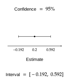
Statistical inference
Normal-mean intervals with KNOWN population sigma: mean +/- z sigma/sqrt(n), using two-sided 90%, 95% or 99% critical values. Five deterministic illustrative samples show coverage of the chosen population mean, not a random coverage experiment. Comparison mode displays four editable estimates with a shared standard error, without meta-analysis pooling. No estimated-sigma t interval or clinical inference.
Download SVG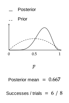
Bayesian inference
Exact beta-binomial updating for an unknown Bernoulli success probability. Positive integer prior shapes update to a+s, b+n-s. Successes are capped at the trial count and the effective count is displayed. Prior/posterior mode compares normalized densities; likelihood/posterior mode normalizes the binomial likelihood over probability before plotting. A common vertical scale preserves relative heights. No arbitrary prior, MCMC or credible-interval solver.
Download SVG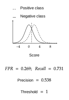
Classification evaluation
Analytic equal-scale logistic score distributions with negative-class location zero and positive-class location d. A threshold determines exact FPR, recall and precision for the specified prevalence. ROC and precision-recall curves follow the same model, including endpoint limits. Density curves and threshold markers are illustrative model predictions, not empirical ROC estimates or fitted classifiers. No unsupported AUC value is reported.
Download SVG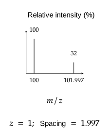
Mass spectrometry
One-chlorine, one-bromine and two-chlorine isotope clusters use fixed natural heavy-isotope fractions 0.2424 and 0.4931 and approximate isotope mass spacings 1.99705 / 1.99795 Da. Two-chlorine intensities are binomial. Isotope intensities normalize to the largest peak. Mass is the user-specified light-isotopologue ion mass, so m/z=ion mass/z; no neutral-mass/adduct correction is inferred. Custom mode provides five editable sticks. This is not fragmentation prediction or a molecular-formula isotope engine.
Download SVG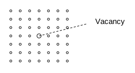
Materials microstructure
Controlled lattice schematics for a vacancy, substitutional atom and an extra half-plane terminating at an edge-dislocation core. The edge lattice relaxes schematically rather than using an elastic displacement solution. Screw mode shows a helical-plane schematic around a line with parallel Burgers-vector direction; it does not depict particles moving on a helix. No atomistic relaxation, defect-energy calculation or crystal-plasticity simulation.
Download SVG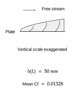
Aerodynamics
Flat-plate laminar scaling delta(L)=5 L/sqrt(Re_L) and mean skin-friction coefficient 1.328/sqrt(Re_L), for the displayed Reynolds-number range. The normalized profile is the Pohlhausen approximation 2 eta-2 eta^3+eta^4, not a numerical Blasius solution. Growing-layer height is vertically exaggerated. Separation is a fixed adverse-pressure-gradient/reverse-flow schematic; no CFD or separation-location prediction.
Download SVG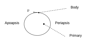
Orbital mechanics
Bound elliptical orbit with primary at a focus, mean anomaly solved by six Newton updates (eccentricity<=0.75), and a tangent velocity direction. Equal-time mode shades sectors with equal mean-anomaly spans at periapsis and apoapsis. Hohmann mode is a coplanar two-impulse transfer between circular orbits, giving total delta-v normalized by the initial circular speed. These are two-body constructions; no N-body propagation or mission optimization.
Download SVG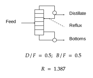
Separation engineering
Ideal binary separation with constant relative volatility and saturated-liquid feed (q=1). Rectifying/stripping lines meet at the feed composition; reflux is a chosen multiple of the feed-pinch minimum, bounded below by 0.5. A maximum of twelve equilibrium steps is drawn, stopping after crossing the bottoms specification; the count reports steps shown. Column mode shows normalized component balances. No multicomponent VLE, enthalpy balance, pressure effects or rigorous column simulator.
Download SVG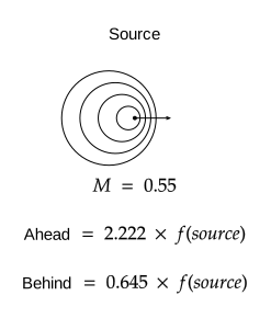
Acoustics
Equal-time spherical wavefront cross-sections for a stationary or uniformly moving point source in a stationary medium. Subsonic on-axis frequency ratios are 1/(1-M) ahead and 1/(1+M) behind. Supersonic mode uses sin(mu)=1/M and tangent cone boundaries. No relativistic Doppler effect, finite-source shock strength or moving-observer calculation.
Download SVG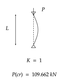
Structural stability
First ideal elastic buckling modes for pinned-pinned, fixed-free and fixed-fixed slender columns. Pcr=pi^2 EI/(KL)^2 with K=1, 2 or 0.5. Young modulus is GPa, second moment is cm^4 and length is metres; the result is kN. Deflection amplitude is illustrative, independent of applied load. No yielding, imperfections, post-buckling or structural design check.
Download SVG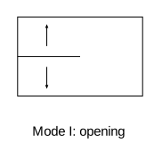
Fracture mechanics
Mode I opening, mode II in-plane sliding and mode III out-of-plane tearing schematics, plus an infinite-plate central crack of total length 2a. The mode-I example uses KI=sigma sqrt(pi a) and plane-stress G=KI^2/E. Stress is MPa, a is mm and E is GPa. No finite-width correction, toughness verdict, crack growth, mixed-mode criterion or safety assessment.
Download SVG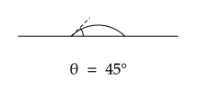
Interfacial physics
A circular-cap drop with its geometric contact angle, signed capillary rise h=2 gamma cos(theta)/(rho g r), or spherical-interface Laplace pressure 2 gamma/r. Gamma is mN/m and radius is mm; density is kg/m^3. The tube meniscus and rise are schematic, while reported values use SI units. A single interface is assumed, not a two-surface soap film. No dynamic wetting or Young-Laplace shape solver.
Download SVG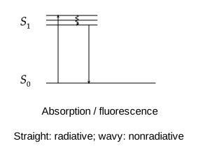
Photophysics
Singlet absorption/fluorescence, triplet intersystem crossing/phosphorescence, or ideal Förster transfer efficiency E=1/[1+(r/R0)^6]. Straight arrows are radiative and wavy paths are nonradiative; relative energy gaps and vibrational spacings are schematic. R0 incorporates the donor-acceptor photophysics. No spectrum, lifetime fit, orientation inference or molecular excited-state calculation.
Download SVG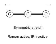
Vibrational spectroscopy
Linear carbon dioxide symmetric stretch, antisymmetric stretch and one of its two degenerate bends. Arrows indicate relative displacement directions at one phase, not calibrated amplitudes or computed eigenvectors. In the harmonic centrosymmetric limit the symmetric stretch is Raman active/IR inactive; antisymmetric stretch and bends are IR active/Raman inactive. No arbitrary-molecule normal-mode solver, frequencies or Fermi-resonance prediction.
Download SVG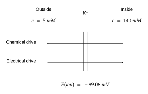
Membrane biophysics
Single-ion equilibrium membrane potential, inside relative to outside: E=(RT/zF) ln(cOutside/cInside). Potassium, sodium and chloride examples use fixed illustrative mM concentrations; custom mode accepts both concentrations and nonzero valence. Opposing arrows indicate balanced chemical/electrical drives, not net equilibrium flux. Ideal dilute activities and a membrane permeable only to that ion; no GHK, channel kinetics or action-potential simulation.
Download SVG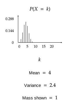
Probability distributions
Exact probability masses for a binomial count, Poisson count or geometric number of failures before the first success. The plot shows k=0 through 24 without renormalizing truncated tails; displayed mass reports the portion shown. Mean and variance describe the full distribution. Independent Bernoulli trials and a constant success probability are assumed. No sampling, fitting or hypothesis testing.
Download SVG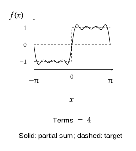
Harmonic analysis
The first one to nine nonzero sine terms for unit-amplitude square, sawtooth and triangle waves on [-pi,pi]. Solid is the exact partial sum and dashed is the target. Odd harmonics are used for square/triangle waves; their displayed term count differs from the highest harmonic. At jumps, Fourier sums tend to the midpoint; square/sawtooth retain Gibbs overshoot. No arbitrary waveform analysis, FFT or data import.
Download SVG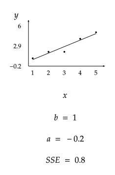
Regression analysis
Ordinary least squares with an intercept for five editable responses at fixed x=1,2,3,4,5. Views show the fit, vertical residuals, or a zero-centered residual plot. The slope, intercept and residual sum of squares are computed from the same data; axes automatically include the observations and fitted endpoints. No confidence bands, causal claim, weighted regression or arbitrary dataset import.
Download SVG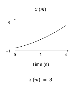
Classical mechanics
Constant-acceleration motion x=x0+v0*t+a*t²/2, v=v0+a*t and a=constant over four seconds. Each view has its own padded vertical scale; position includes an interior turning point when present. The marker uses selected time. SI units; no arbitrary force law, relativistic motion or numerical trajectory solver.
Download SVG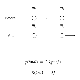
Momentum conservation
Two isolated masses with signed velocities undergo an elastic collision, stick together, or have a chosen coefficient of restitution e. Momentum is conserved; v2'-v1'=e*(u1-u2). Arrows share a velocity scale and point in the signed direction. Rows are before/after states, not simultaneous spatial trajectories. No oblique collision, deformation history or contact-force simulation.
Download SVG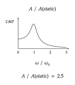
Mechanical dynamics
Steady sinusoidal forcing of a viscously damped oscillator. Amplitude relative to static displacement is 1/sqrt[(1-r²)²+(2*zeta*r)²]; lag=atan2(2*zeta*r,1-r²). Relative dissipated power is (2*zeta*r*A)². Damping is strictly positive. Views use frequency ratio r=omega/omega0, not time; no startup transient or nonlinear resonance.
Download SVG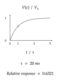
Circuit dynamics
Ideal RC charging/discharging capacitor voltage or RL turn-on current, normalized to the final/initial magnitude. Tau=R*C for RC and L/R for RL; dimensionless time u=t/tau. RC uses kOhm and microfarad, RL ohm and mH, giving tau in ms. No RLC response, switch parasitics, source loading or measured data.
Download SVG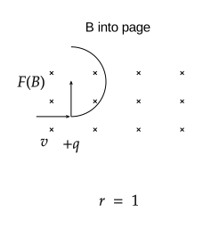
Electromagnetism
A unit-magnitude signed charge enters rightward in a uniform magnetic field into the page. Magnetic force bends positive charges upward and negative downward. A crossed-field selector has E downward and B into the page: undeflected speed is E/B. The circle auto-fits the schematic; radius readout is m*v/(|q|B) in relative units. Nonrelativistic schematic; no helical 3D trajectory, fringe fields or accelerator solver.
Download SVG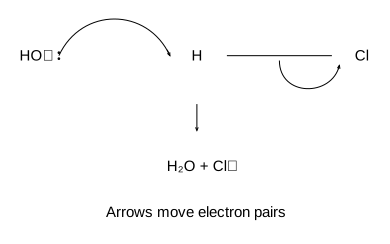
Organic chemistry
Authored elementary proton transfer (hydroxide + HCl), SN2 substitution (hydroxide + methyl bromide), or hydroxide addition to formaldehyde. Curved full-head arrows move electron pairs from donor to electrophile and from the breaking bond to its atom. Only the shown elementary step is represented; the carbonyl product is the alkoxide before protonation. No general molecule editor, mechanism inference or stereochemical simulation.
Download SVG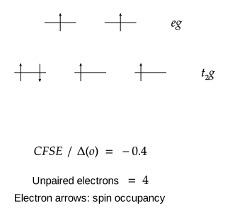
Coordination chemistry
Octahedral d6 high-spin or low-spin occupations, or tetrahedral e/t2 splitting without an electron-filling example. Octahedral levels are -0.4Delta and +0.6Delta; tetrahedral levels -0.6DeltaT and +0.4DeltaT, DeltaT/DeltaO=4/9 for the ideal comparison. CFSE excludes pairing energy. Arrows are electron spin, not transitions. No arbitrary ligand-field calculation or spectrochemical prediction.
Download SVG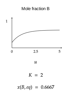
Chemical equilibrium
Ideal closed first-order A <-> B with equilibrium ratio K=B/A=kForward/kReverse and total fraction A+B=1. Time u=(kForward+kReverse)t. Views show relaxation, DeltaG/RT=ln(Q/K), or a change in initial fraction at unchanged K. Changing initial amounts changes the approach, not the equilibrium ratio. No arbitrary reaction, activity corrections or temperature/pressure equilibrium solver.
Download SVG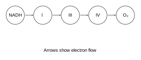
Cellular energetics
Qualitative mitochondrial electron transport (NADH -> I -> III -> IV -> O2), proton-gradient-driven ATP synthase, or linear photosynthetic flow (H2O -> PSII -> chain -> PSI -> NADP+). Intermediate carriers are omitted in the abbreviated tracks. ATP synthesis uses proton return; no quantitative proton/ATP yields, free-energy scale, full Calvin/Krebs cycle or biochemical simulation.
Download SVG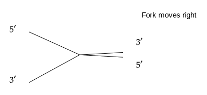
Molecular biology
A right-moving replication fork with antiparallel parental strands. The lower template runs 3' to 5' toward the fork, supporting continuous 5' to 3' leading synthesis. Upper-template Okazaki fragments grow away from the fork, each 5' to 3'. A separate ligation view joins adjacent fragments after primer replacement. No nucleotide sequence, helicase kinetics or complete replisome model.
Download SVG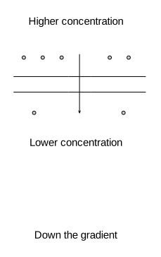
Membrane transport
Qualitative transport across a membrane with higher solute concentration above and lower below. Simple diffusion crosses lipid; facilitated diffusion uses a channel; an ATP-driven pump transports upward against the shown concentration gradient. Dot counts only indicate relative concentration, not flux or stoichiometry. No electrochemical potential, specific sodium-potassium cycle or osmotic-pressure solver.
Download SVG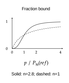
Biophysical binding
Normalized Hill binding S=p^n/(P50^n+p^n), where the pressure axis is p divided by a reference P50. Compare n=1 and n=2.8, shift P50, or mark high/low pressures and their saturation difference. This is an ideal illustrative binding model, not an individual blood-gas curve or clinical interpretation. No temperature/pH calibration or gas-exchange physiology solver.
Download SVG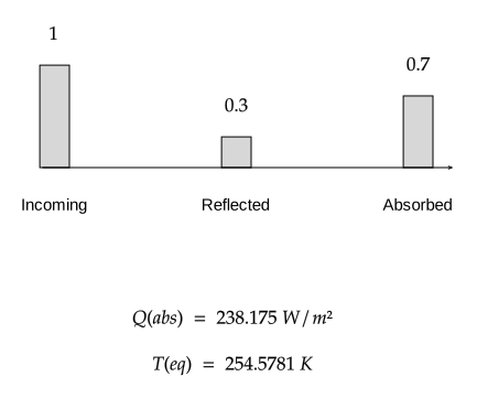
Climate physics
Ideal global-mean energy balance with incoming S/4, reflected alpha*S/4 and absorbed (1-alpha)*S/4. Bare-planet Te=[absorbed/sigma]^1/4. A solar-transparent, infrared-gray atmospheric layer gives Ts=Te/(1-epsilon/2)^1/4. Arrows show paths, not measured flux proportions. No convection, clouds, spectral atmosphere or forecast. Temperatures are ideal equilibrium kelvin.
Download SVG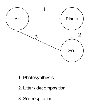
Biogeochemical cycles
Qualitative selected carbon pathways: atmosphere-plants-soil biological loop, atmosphere/surface/deep-ocean exchanges, or photosynthesis-burial-combustion through fossil storage. Intermediate reservoirs/processes are omitted. Bidirectional ocean links indicate exchange, not equal measured fluxes. No quantitative global budget, residence times, climate feedback or future emissions scenario.
Download SVG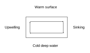
Oceanography
Schematic basin overturning, offshore-wind coastal upwelling, or normalized thermocline/halocline profiles. The profiles are T=exp(-z/h) and S=1-0.7exp(-z/h), with increasing depth downward: qualitative structure, not seawater EOS or observations. Overturning is a two-dimensional conceptual cell, not a geographic current map or quantitative circulation forecast.
Download SVG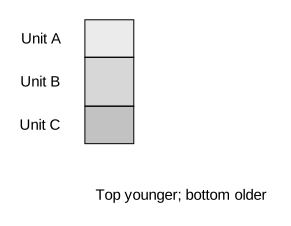
Geology
Three ordered sedimentary units, two-column lithostratigraphic correlation, or a schematic angular unconformity with tilted beds below an erosion surface and horizontal younger beds above. Layer heights use relative thickness with a font-aware minimum for readable labels; drawings are not a surveyed depth scale. No age inference, geologic map projection or quantitative sedimentation model.
Download SVG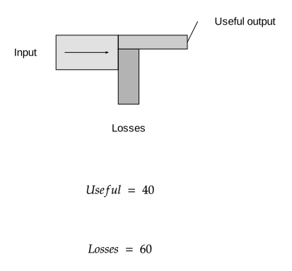
Energy engineering
Normalized conserved-width energy streams. Input is 100 units; useful output is eta, losses 1-eta. Cogeneration splits the remainder into useful heat and waste. Two-stage conversion has useful fraction eta1*eta2 and combined losses. Band widths, not areas or lengths, encode flow. Not measured national energy data or an unrestricted Sankey layout engine.
Download SVG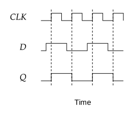
Digital systems
Positive-edge D-flip-flop timing with Q initially zero, two-bit binary count on the same clock edges, or a three-state Moore cycle. Data changes precede clock edges; Q changes only at rising edges. Ideal zero-delay logic: no setup/hold violations, metastability or waveform simulation. State labels show state/output; each directed transition is one clock event.
Download SVG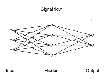
Machine learning
Editable schematic 3-4-2 dense network, input-convolution-pooling-dense chain, or a residual block y=F(x)+x. Connection lines in the dense network denote weights, not inferred importance; no training or data-dependent architecture generation. Block sizes are schematic, not tensor dimensions. The residual sum has matching input/output dimensions by assumption.
Download SVG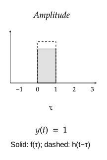
Signals and systems
Unit-width rectangular pulses convolve to y(t)=max[0,min(1,t)-max(0,t-1)]. The overlap view shows f(tau) and shifted h(t-tau). Other views show h(t)*tau=exp(-t/tau) or the unit-step response 1-exp(-t/tau) of an ideal causal first-order low-pass system. No arbitrary convolution, numerical filtering or startup delay.
Download SVG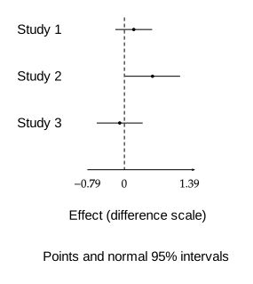
Research methods
Three estimates with normal 95% intervals, six fixed-mean paired differences with bias and descriptive limits mean±1.96 sample SD, or fixed-effect inverse-variance pooling of the estimates. Agreement means are illustrative fixed x=1..6; pooled uncertainty assumes independent estimates and known SEs. No random-effects meta-analysis, clinical equivalence judgment or inference from real study data.
Download SVG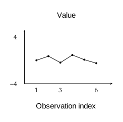
Statistical diagnostics
Six editable observations form a run-sequence plot or standardized individual values against known center and sigma with ±3 reference limits. These are not estimated control limits or a process-capability claim. The separate AR(1) panel shows theoretical rho(k)=rho^k for |rho|<1, not sample autocorrelations or confidence bands. No forecasting, AR fitting or automatic alarm decisions.
Download SVG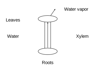
Plant physiology
Qualitative xylem water flow from roots to leaves and atmosphere; phloem source-to-sink sugar transport with loading/unloading; or an open stoma with CO2 entry and water-vapor loss. Phloem direction is source-to-sink, not universally downward. Shapes are symbolic, not leaf anatomy or a quantitative water-potential/pressure-flow model.
Download SVG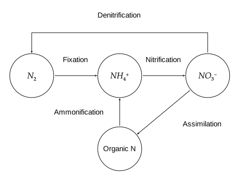
Biogeochemistry
Selected microbial/plant nitrogen pathways: N2 fixation to ammonium, nitrification to nitrate, assimilation into organic nitrogen, ammonification and denitrification back to N2. Separate views isolate two-step aerobic nitrification and plant recycling. Arrows show transformations, not measured fluxes. Intermediate organisms and other pathways such as anammox are omitted.
Download SVG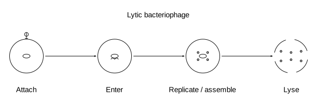
Virology
Four-stage authored tracks: lytic bacteriophage attachment through lysis; temperate-phage integration, host division and induction into the lytic cycle; or a positive-strand RNA virus entering, translating, copying RNA and releasing progeny. Stages are abbreviated and virus-specific, not universal replication rules. Cells/virions are symbols, not molecular structures or an infection simulation.
Download SVG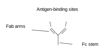
Immunology
Symbolic IgG with two Fab antigen-binding arms and an Fc stem; bivalent binding to matching epitopes; or antibody cross-linking between antigen-bearing particles. Y shapes summarize heavy/light-chain organization. Binding is schematic, not affinity kinetics, a structural protein model, immune-response prediction or a claim that every antibody is a monomeric IgG.
Download SVG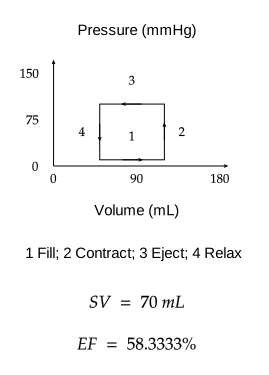
Cardiovascular physiology
An ideal rectangular left-ventricular pressure-volume loop: filling, isovolumetric contraction, ejection and isovolumetric relaxation. Separate pressure/volume tracks use equal illustrative phase durations. Stroke volume is EDV-ESV; EF is SV/EDV. Corner pressures and durations are idealizations, not a clinical Wiggers diagram, patient data or diagnostic model.
Download SVG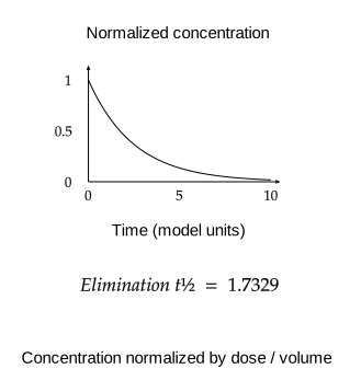
Pharmacokinetic models
Normalized one-compartment first-order models: IV bolus elimination, absorption with elimination, or three equal boluses with instantaneous concentration jumps. Absorption handles equal absorption/elimination rates by its analytic limit. Time and concentration are model units; no drug, dose recommendation, bioavailability fitting, patient calibration or multicompartment physiology is implied.
Download SVG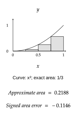
Calculus
Left, right or midpoint rectangles approximate the integral of x² on [0,1], with exact finite-sum area and signed error against 1/3. A separate view compares exp(x) with its Maclaurin polynomial of order 1–5 on [-1,1]. These are exact authored examples, not an arbitrary symbolic integration or Taylor-series engine.
Download SVG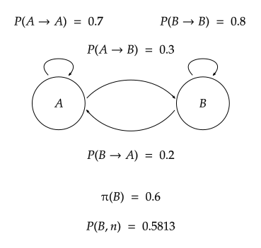
Stochastic processes
Two-state transition graph, discrete probability evolution, or an absorbing B state. p=P(A→B), q=P(B→A); b(n+1)=p+(1-p-q)b(n). The stationary B probability is p/(p+q), with q=0 in the absorbing view. Initial B probability and step count are editable. This is a two-state homogeneous example, not a general transition-matrix, hidden-state or inference tool.
Download SVG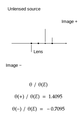
Gravitational astronomy
Thin point-mass lens in Einstein-angle units: source offset beta gives images theta±=(beta±sqrt(beta²+4))/2. Views show collinear sky-plane positions, the lens mapping beta=theta-1/theta on separate branches, or a perfectly aligned Einstein ring. Positions are angular, not physical ray paths. No extended mass profile, cosmological distance calculator or full gravitational ray tracing.
Download SVG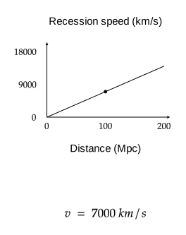
Cosmology
Low-redshift v=H0 d, uniform expansion between two illustrative epochs, or cosmological wavelength stretching lambda(observed)/lambda(emitted)=a(observed)/a(emitted)=1+z. Galaxy positions are schematic comoving markers. The Hubble plot is a low-z relation, not a relativistic recession-speed estimator or a fitted cosmological expansion history; peculiar velocities are omitted.
Download SVG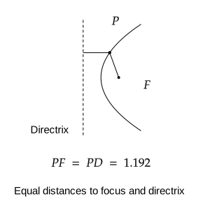
Analytic geometry
A parabola with focus/directrix and equal distances, an ellipse with two focal distances summing to 2a, or a hyperbola with focal-distance difference 2a and asymptotes. Ellipse a=2; hyperbola a=b=1. Points follow the actual curves. This complements orbital ellipses and generic curve drawing; it is not a general quadratic parser or rotated-conic solver.
Download SVG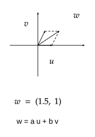
Linear algebra
An oblique basis u=(1,0), v=(s,1); kernel and range of A(x,y)=(x+s y,0); or the affine solution line x+s y=c parallel to the nullspace. Coordinates and particular solutions are computed for these exact 2D examples. This adds explicit subspace/solution geometry beyond SVD and projection presets; it is not an arbitrary matrix or linear-system solver.
Download SVG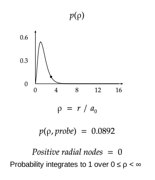
Atomic quantum physics
Normalized radial probability p(rho) for hydrogen 1s, 2s or 2p, with rho=r/a0 and probability p(rho)d(rho). The 2s radial node is rho=2; 1s and 2p have no positive radial nodes. Curves are shown to rho=16, while normalization is over [0,infinity). This is radial probability, not the spatial density |psi|² or an electron trajectory; angular shapes and multi-electron atoms are omitted.
Download SVG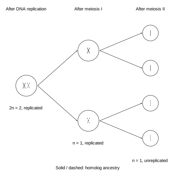
Genetics and cell biology
A 2n=2 example separates homologs in meiosis I and sisters in meiosis II; a separate four-chromatid example exchanges segments between nonsisters. Independent-assortment view gives four equally likely gamete classes across many meioses of AaBb with unlinked loci, not four classes from each single meiosis. Solid/dashed ancestry is symbolic; no detailed spindle, molecular crossover or arbitrary karyotype engine.
Download SVG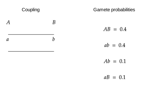
Genetic linkage
Coupling AB/ab and repulsion Ab/aB produce parental gametes (1-r)/2 each and recombinant gametes r/2 each. A three-locus map uses Haldane r=(1-exp(-2d))/2, d in Morgans, with additive map distances; pairwise recombination fractions are not additive. This assumes no crossover interference for the map model. No empirical inference, double-crossover counting or clinical genetic prediction.
Download SVG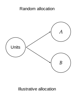
Experimental design
Two-treatment allocation schematics: completely randomized allocation from a common pool, one A and one B randomized within each matched pair, or balanced A/B assignments within each block. A/B are editable treatment labels. Fixed balanced arrangements illustrate structure and are not freshly randomized assignments, an outcome analysis, sample-size calculation or clinical protocol.
Download SVG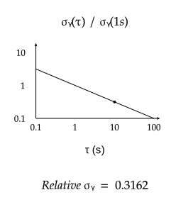
Frequency metrology
Ideal normalized Allan-deviation power laws for white frequency noise (tau^-1/2), flicker frequency noise (constant), and random-walk frequency noise (tau^1/2). Both axes are logarithmic; sigma is normalized to its value at one second. These are asymptotic signatures, not estimates from time-series data or confidence intervals. No phase-noise conversion or real clock characterization.
Download SVG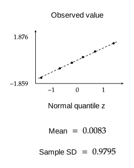
Distribution diagnostics
Six ordered observations are paired with standard-normal quantiles at (i-0.5)/6. The dashed reference is sample mean plus sample standard deviation times z; it is not a fitted regression or a normality test. Presets show normal-like, heavy-tail and right-skew patterns; custom observations are sorted. Constant samples remain valid horizontal plots. No p-values or large-data import.
Download SVG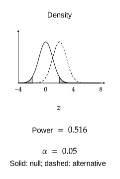
Statistical inference
Known-standard-error Gaussian Z tests with two-sided or upper one-sided alternatives. Alpha selects tabulated standard-normal critical values. The alternative mean is delta standard errors above zero; power integrates the shown rejection tails using a bounded normal-CDF approximation. The power-curve view is two-sided. Illustrative planning model only: no unknown-variance t test, sequential testing or data fitting.
Download SVG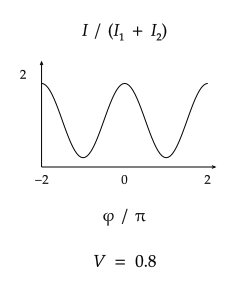
Statistical optics
Two-beam interference normalized by I1+I2: I=1+V*cos(phi), V=2*sqrt(r)/(1+r)*|gamma|, with r=I2/I1. Views show fringes, intensity-balance contrast or a Gaussian temporal-coherence envelope exp[-(delay/tauC)²/2]. Gamma is a magnitude in [0,1]. No spatial propagation, Fourier reconstruction, measured spectrum or coherence-time estimation.
Download SVG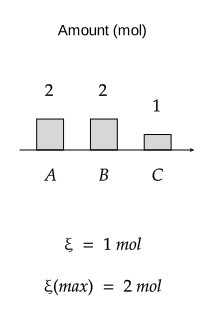
Reaction stoichiometry
Fixed balanced reaction 2A+B -> C. Extent xi runs from zero to min(nA0/2,nB0); remaining species follow nA=nA0-2xi, nB=nB0-xi, nC=nC0+xi. Views show amounts, the A-B composition path or maximum extent as initial A varies. No automatic balancing, kinetics, equilibrium or gas-volume assumption. Amounts are moles.
Download SVG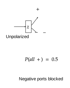
Quantum measurement
Unpolarized spin-1/2 input is filtered through the positive output of one, two or three analyzers: z, then an axis at theta, then z again. Conditional positive probability is cos²(theta/2); joint throughput is 1/2, (1/2)cos² or (1/2)cos^4. Negative outputs are blocked, not recombined. Schematic spatial paths do not model field forces or coherent beam recombination.
Download SVG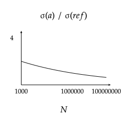
Fatigue mechanics
Illustrative normalized fatigue models: Basquin stress amplitude sigma/sigmaRef=(N/10^6)^b; Goodman line sigmaA/sigmaE=1-sigmaM/sigmaU for tensile mean stress; or Palmgren-Miner damage D=sum(ni/Ni). These ideal relations omit scatter, sequence effects, residual stress and material calibration. A point below the Goodman line is only below this model boundary, never a safety or life prediction.
Download SVG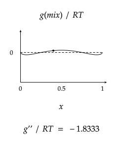
Solution thermodynamics
Symmetric regular solution gMix/RT=x ln(x)+(1-x)ln(1-x)+chi*x(1-x), with endpoint limits. Views show free energy, the spinodal T/Tc=4x(1-x), or partial mixing chemical potentials. Chi=Omega/RT; spinodal markers use T/Tc=2/chi where within view. The spinodal is a local-curvature boundary, not the coexistence binodal. No common-tangent or multicomponent equilibrium solver.
Download SVG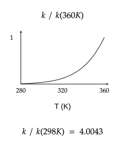
Chemical kinetics
Arrhenius rates normalized to their value at 298 K, with activation energy in kJ/mol. The temperature view plots k(T)/k(360K); the inverse-temperature view plots ln[k(T)/k(298K)]. Two pathways share a reference ratio kB/kA at 298 K and are normalized by a common maximum. Constant activation energies, no fitted data, tunneling, temperature-dependent prefactors or Eyring transition-state calculation.
Download SVG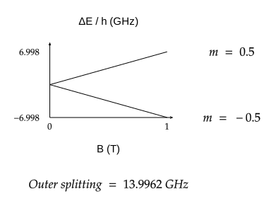
Atomic spectroscopy
Linear weak-field Zeeman shifts DeltaE/h=g*muB*mJ*B/h, with muB/h=13.99624555 GHz/T. J=1/2,1 or3/2 gives two, three or four magnetic sublevels. All levels coincide at B=0. The plotted fan rescales to the chosen field endpoint. No hyperfine structure, transition strengths, selection rules or strong-field Paschen-Back regime.
Download SVG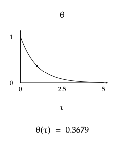
Transient heat transfer
Lumped Newton cooling theta=exp(-tau), or exact one/two-mode solutions of a constant-diffusivity rod with zero-temperature endpoints. Fo=alpha*t/L²; the second initial profile is sin(pi*x/L)+0.3sin(3pi*x/L). Solid is the selected state and dashed the initial rod profile. Lumped time uses its thermal time constant. No arbitrary initial data, convection boundary solver or temperature-dependent properties.
Download SVG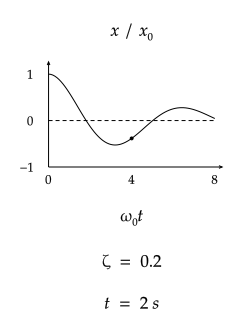
Mechanical dynamics
Exact free response x''+2*zeta*x'+x=0 in tau=omega0*t, starting at x/x0=1 and zero velocity. The three views use underdamped, critically damped and overdamped forms; the overdamped expression avoids growing intermediate exponentials. Omega0 is rad/s. No forcing, nonlinear spring, friction law or fitted experimental response.
Download SVG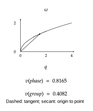
Dispersive waves
Normalized model relations omega=sqrt(q), omega=q and omega=q² illustrate deep-water-like, nondispersive and free-particle-like behavior. Phase velocity is omega/q and group velocity is d(omega)/dq at the marker. The dashed local tangent and solid origin-to-marker secant show these slopes. Units are normalized; no finite-band packet evolution or arbitrary medium model.
Download SVG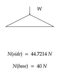
Cable and truss mechanics
A symmetric pin-jointed triangular truss under a vertical apex load, a parabolic cable loaded uniformly per horizontal length, or a self-weight catenary. Truss member forces are exact for its shown aspect ratio. Cable drawings normalize horizontal/vertical scales separately; H=w*b²/(2f) for a parabola and H=w*a for a catenary. No arbitrary truss network, extensibility, distributed-wind or structural design check.
Download SVG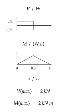
Beam mechanics
Ideal Euler-Bernoulli examples: simply supported central point load or uniform load, with normalized shear/moment diagrams; or a cantilever with end force and normalized deflection. W is total applied load. Physical extrema use kN, m, GPa and cm^4, with tip deflection in mm. Small-deflection, constant-EI assumptions; no arbitrary loading, shear deformation, yielding or design assessment.
Download SVG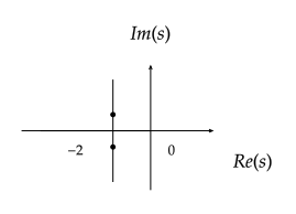
Feedback control
The roots of s²+2s+K trace a real-to-complex locus, with damping ratio 1/sqrt(K) for K>0. A separate cubic s³+3s²+2s+K has Routh first column 1,3,(6-K)/3,K: strict stability requires 0<K<6. Zero or six are marginal boundaries. These fixed polynomials illustrate pole migration and the Routh criterion; no arbitrary transfer-function solver.
Download SVG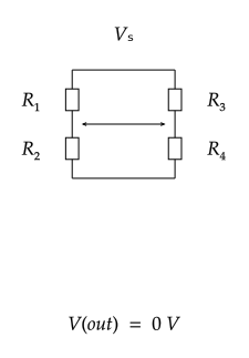
Electrical measurement
An ideal unloaded Wheatstone bridge has Vout=Vleft-Vright=Vs[R2/(R1+R2)-R4/(R3+R4)]. The quarter bridge changes R1=R(1+delta), giving Vout/Vs=1/(2+delta)-1/2, with small-change approximation -delta/4. Curves compare the exact response and linear approximation. No lead resistance, temperature compensation or instrument loading.
Download SVG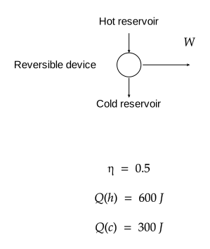
Thermal machines
Ideal reversible engine or refrigerator between Th>Tc. Engine efficiency is 1-Tc/Th; refrigerator COP=Tc/(Th-Tc). W is positive work magnitude. The Carnot T-s rectangle has width deltaS=W/(Th-Tc), Qh=Th*deltaS and Qc=Tc*deltaS. Temperatures are kelvin, energies joules. This is an ideal limit, not a prediction of actual machine performance.
Download SVG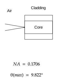
Guided-wave optics
Ideal circular step-index fiber in air: NA=sqrt(ncore²-nclad²), acceptance half-angle=asin(NA), V=2*pi*a*NA/lambda. The weak-guidance single-mode boundary is V=2.405. Views show an acceptance cone, index profile or V versus core radius. Rays are schematic; no Bessel-mode solver, bend loss, graded index or wavelength-dependent indices.
Download SVG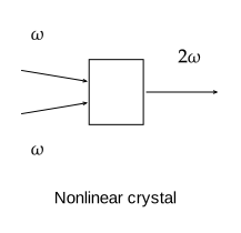
Nonlinear optics
Undepleted second-harmonic generation: two input photons at omega produce one at 2omega. Relative conversion follows sinc²(deltaK*L/2), using q=deltaK*L/(2*pi). A periodically poled domain sketch illustrates sign reversal of the quadratic coefficient d, not a material-specific efficiency model. No pump depletion, dispersion solver, focusing or quasi-phase-matching optimization.
Download SVG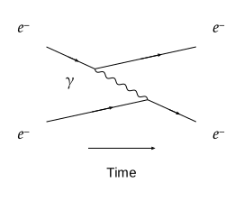
Particle physics
Editable QED examples with time from left to right: one electron-electron exchange diagram, electron-positron to muon-pair annihilation, or one Compton s-channel diagram. Fermion arrows show charge flow; antiparticle arrows oppose physical propagation. Wavy lines are photons. These are individual contributions, not complete amplitudes, cross sections, particle trajectories or automatic diagram generation.
Download SVG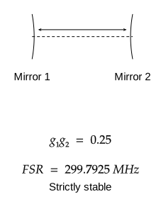
Laser engineering
Two-mirror paraxial cavity with g_i=1-L/R_i, a g1-g2 stability map, or five longitudinal resonances relative to a reference mode. Strict stability is 0<g1*g2<1; boundaries are marked marginal and can be degenerate. FSR=c/(2nL) assumes a nondispersive uniform index. Mirror curvature is schematic. No Gaussian eigenmode, misalignment, gain or real-cavity stability solver.
Download SVG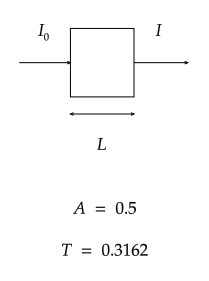
Absorption spectroscopy
Ideal monochromatic absorption with A=epsilon*c*L and transmission 10^(-A). Epsilon uses L mol^-1 cm^-1, concentration is micromolar and path length is cm. Views show a schematic cuvette, linear absorbance calibration, or intensity along the path. Beam arrow lengths are schematic. No scattering, stray light, saturation, chemical speciation or fitted experimental calibration.
Download SVG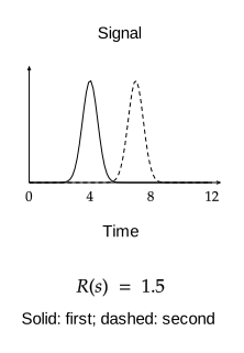
Separation performance
Two equal-height Gaussian peaks with common sigma, resolution Rs=deltaT/(4 sigma) using baseline widths 4 sigma, or H=A+B/u+C*u with positive coefficients. The normalized Van Deemter view reports u(opt)=sqrt(B/C) and H(min)=A+2sqrt(BC). No measured peak fitting, tailing, gradient elution or instrument optimization. Curves use internally consistent relative time/velocity/plate-height units.
Download SVG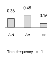
Population genetics
One biallelic locus with random mating: AA=p², Aa=2p(1-p), aa=(1-p)². Selection view reweights these genotype frequencies by positive relative viabilities and reports the surviving allele frequency p(next). Survivor genotypes need not be Hardy-Weinberg proportions. No drift, migration, mutation, linkage, lethal-fitness boundary or empirical inference.
Download SVG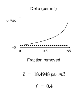
Isotope geochemistry
Trace-isotope Rayleigh model with constant alpha=R(instantaneous product)/R(reservoir). Residual ratio is R0*f^(alpha-1); accumulated product is R0*(1-f^alpha)/(1-f), using its alpha limit at f=1. Delta values are per mil relative to a standard. The mixed reservoir continuously loses product without re-equilibration. No measured isotope fit or multi-reservoir mass-balance solver.
Download SVG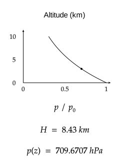
Atmospheric physics
Ideal isothermal hydrostatic pressure p/p0=exp(-z/H), H=Rd*T/g, and constant-lapse environmental/dry-parcel temperature profiles. Dry lapse is g/cp with Rd=287.05 and cp=1004 J/(kg K). A selected-height parcel compares temperatures at equal pressure; positive difference means dry instability. No moisture, entrainment, real weather forecast or standard-atmosphere fit.
Download SVG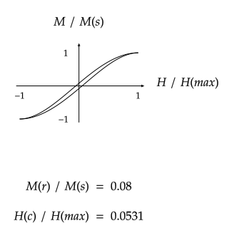
Magnetic materials
Closed normalized illustrative loops m=(3h-h^3)/2 +/- r(1-h^2)^2, with flat saturated endpoints at h=+/-1 and positive branch slopes for r<=0.35. Soft and hard examples differ in loop width. Remanence is r; coercivity is solved on the same upper branch. The model is schematic, not a measured material law, minor-loop model, energy-loss calibration or magnet design tool.
Download SVG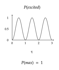
Coherent quantum dynamics
Driven two-level probabilities in the rotating-wave approximation: P=sin²(pi*tau) on resonance and P=sin²(pi*sqrt(1+d²)*tau)/(1+d²) with d=detuning/Rabi frequency. Tau counts resonant Rabi periods. Avoided crossings use eigenvalues +/-sqrt(delta²/4+g²) of a real two-state Hamiltonian. No decoherence, many-level dynamics, sweep transition probabilities or pulse simulation.
Download SVG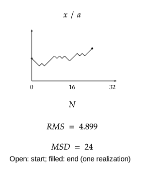
Stochastic processes
Three fixed seeded examples of symmetric one-dimensional or cardinal-step two-dimensional walks, plus the ensemble relation mean-square displacement=N*a² for independent steps of length a. The selected path is not an ensemble estimate and does not re-randomize. Axes use step counts/step-length units; RMS and MSD use the chosen a. No stochastic differential-equation solver or uncertainty inference.
Download SVG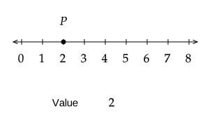
Mathematics
Counting, rational numbers, directed jumps, open/closed intervals and aligned double number lines. Positions use exact equal steps. Worksheet mode hides the marked value or jump result, retaining the scale.
Download SVG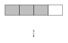
Mathematics
Equal-part bars, circles or rectangular grids, including multiple wholes. Grid denominator is columns × rows. Answers can use improper, mixed-number or equivalent-fraction notation; worksheet mode leaves an answer line.
Download SVG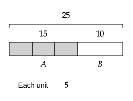
Mathematics
Part–whole, comparison and ratio bars share one unit length. Unit value is given; worked mode shows the resulting totals and difference. Worksheet mode retains the bars and given unit value.
Download SVG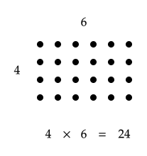
Mathematics
Equal rows and columns as dots, a unit grid or a partitioned rectangle. A common unit size preserves the multiplication model. Worksheet mode hides the product while retaining row/column counts.
Download SVG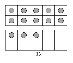
Mathematics
Two ten frames, grouped counters or base-ten hundreds/tens/ones. Counters and blocks preserve their counts. Worksheet mode hides the written total and place-value answers.
Download SVG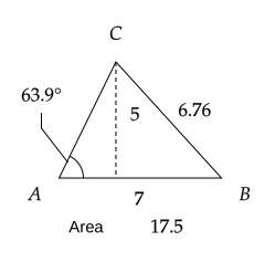
Mathematics
Dimensioned right/isosceles/scalene triangles, rectangles, parallelograms and circles. Computed sides, angles and areas follow the given dimensions. Figures are schematic; angles use the actual construction. Worksheet mode hides derived answers, retaining given dimensions.
Download SVG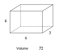
Mathematics
Dimensioned cube, cuboid, right-triangular prism and square pyramid, each with a fixed valid net. Dashed edges are hidden edges or folds. Lengths determine volume/surface area; perspective views are schematic. No arbitrary unfolding is attempted.
Download SVG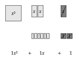
Mathematics
Signed algebra tiles (light positive, dark crossed negative), an equation balance, or an (x+a)(x+b) area model. Balance tilt compares the two expressions at the specified x; it does not solve an equation. Factoring layouts use positive integer a and b.
Download SVG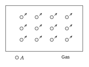
Chemistry
Solid, liquid and gas arrangements for one element, an unbonded A/B mixture or identical bonded AB molecules. The count means particles for elements/mixtures and molecules for AB. State changes preserve that count; positions and motion arrows are schematic, not a molecular simulation.
Download SVG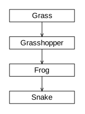
Biology
A three-to-five-organism chain or an editable six-organism food web. Arrows point from food/resource to the consumer, including transfer to decomposers. The presets illustrate energy transfers, not an energy cycle or population model. Worksheet mode leaves organism boxes blank.
Download SVG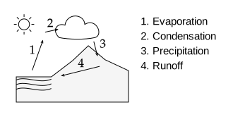
Earth science
A schematic ocean–land water cycle. The simple view has four processes; the detailed view adds infiltration, groundwater flow and transpiration. Numbers connect the drawing to editable process labels. Worksheet mode blanks that legend. Storage and fluxes are not to scale.
Download SVG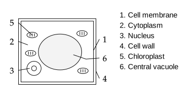
Biology
Schematic plant, animal and bacterial cells with numbered organelle callouts. Simple mode retains the main distinguishing structures; detailed mode adds ribosomes and selected organelles. Bacteria have a nucleoid, not a nucleus. Shapes and relative sizes are illustrative, not microscopy or scale drawings.
Download SVG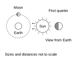
Earth science
Separate teaching views: lunar phases (orbit view plus Earth-observer appearance), aligned solar/lunar eclipses, two solstices, and day/night from above the north pole. Eclipse presets assume alignment near an orbital node, not an eclipse every month. Sizes/distances are schematic; seasons come from axial tilt.
Download SVG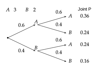
Statistics
Two draws from an A/B collection, with or without replacement, or an equally likely 1…n × 1…n sample-space grid. Grid cells show sums. Branch and joint probabilities are calculated and rounded to three decimals; worksheet mode hides probabilities/cell answers while retaining given counts and headers.
Download SVG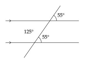
Mathematics
Intersecting lines or parallel lines cut by a transversal. The given angle determines supplementary, vertically opposite and corresponding angles. Worksheets retain the given angle and show unknowns.
Download SVG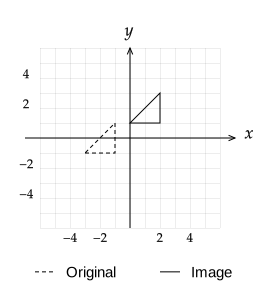
Mathematics
A triangle and its image under translation, reflection, rotation or positive enlargement. Rotation and enlargement are about the origin. Dashed outlines show the original; worksheets hide the image.
Download SVG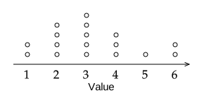
Statistics
Dot plots use frequencies at values 1–6. Histograms use six unit-width bins [0,1), …, [5,6]. Box plots use five editable observations; quartiles are medians of the two halves excluding the overall median, with min/max whiskers.
Download SVG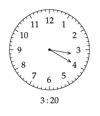
Mathematics
An analog clock with a continuously geared hour hand, a centimetre ruler with millimetre marks, or a semicircular protractor. The worked reading can be hidden for worksheets.
Download SVG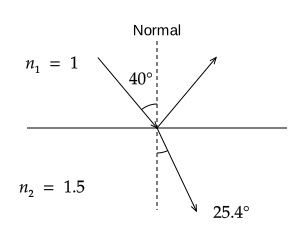
Physics
A plane mirror or two transparent media. Angles are measured from the normal. Snell’s law determines the transmitted ray, including the critical angle and total internal reflection; reflected intensity is not calculated.
Download SVG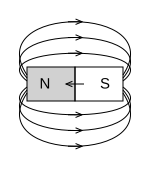
Physics
Schematic field lines for a bar magnet, a solenoid or a straight wire viewed end-on. Arrows form closed magnetic paths; reversing poles/current reverses every field arrow. A dot means current out of the page and a cross means into it. Field strength and arbitrary sources are not solved.
Download SVG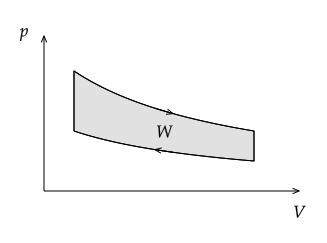
Physics
Relative pressure–volume diagrams: isobaric, isochoric, ideal-gas isothermal, rectangular cycle or Stirling cycle. Shading is work by the gas (the enclosed area for a cycle). Isotherms obey pV = constant; axes are relative, without claimed material data.
Download SVG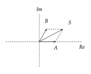
Engineering
Two phasors and their vector sum, or series-RLC voltage phasors using current as the horizontal reference. Inductive voltage leads current by 90° and capacitive voltage lags by 90°. Amplitudes use one scale; this is a static snapshot, not a circuit solver.
Download SVG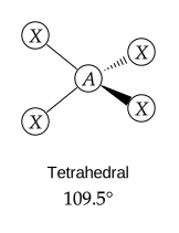
Chemistry
Curated 2D projections of seven molecular geometries, with solid/hashed wedges for depth and ideal 3D angle guides. Bent and pyramidal presets use four electron regions with lone pairs; their angles are below 109.5°. Labels do not infer element valence or a molecule’s exact geometry.
Download SVG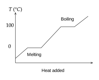
Chemistry
A pure-substance heating/cooling curve at constant pressure, with melting/freezing and boiling/condensation plateaus. Heat-axis segment widths are schematic, not material heat capacities or latent heats. A time axis assumes constant heating/cooling power.
Download SVG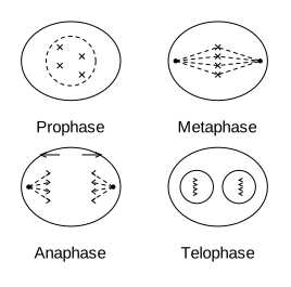
Biology
Schematic animal-cell mitosis: one stage or a four-panel sequence. Prophase includes simplified nuclear-envelope breakdown. Each X is a replicated chromosome; anaphase separates its sister chromatids. Each daughter retains 2n chromosomes. Interphase and cytokinesis are shown separately from mitosis.
Download SVG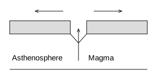
Earth science
Divergent and oceanic–continental convergent boundaries in cross-section, or a transform boundary in plan view. Arrows show relative plate movement. Subduction angle and plate separation are schematic; this is not a geodynamic or earthquake model.
Download SVGNo figures match these filters. Try a different term or clear the filters.